library(dplyr)
library(ggplot2)
library(sf)
library(terra)
library(tidyterra)Reclassify CDL
Here are some geoprocessing examples for reclassifying the cropland data layer (CDL) data from BeeSpatial. BeeSpatial provides forage, nesting, and insecticide rasters as buffered summaries using distance-weighted means of 1, 3, and 5km radius buffers. This means that each pixel of the raster represents the distance-weighted mean of the index values within the corresponding buffer radius.
However, if you only need forage, nesting, or insecticide values themselves instead of buffer summaries, you can obtain this through reclassifying the CDL. This tutorial shows how to do that.
First, load the necessary packages. More info on these packages and their installation can be found here.
Read in the CDL data downloaded from BeeSpatial.
centre_cdl <- rast("data/CDL_2021_FIPS_42027.tif") # change the filepath to reflect where you've stored the dataReclass crop land cover to spring floral resources
The CDL raster values are numeric codes that represent crop land cover class from the CDL. We can reclassify these CDL values to the estimated floral resources of each land cover class, based on Koh et al. (2015).
A formatted reclassification table based on Koh et al. is available here. The table rows connect each CDL value to its corresponding class name and the values for several indices.
reclass_table <- read.csv("data/cdl_reclass_koh.csv")  # read in the reclassification table

head(reclass_table)     # take a look at the first 5 rows
value class_name nesting_ground_availability_index
1 0 Background 0.0000000
2 1 Corn 0.1451854
3 2 Cotton 0.3355898
4 3 Rice 0.1513067
5 4 Sorghum 0.1451854
6 5 Soybeans 0.1993286
nesting_cavity_availability_index nesting_stem_availability_index
1 0.00000000 0.0000000
2 0.08947642 0.1069437
3 0.22867787 0.2335293
4 0.13945144 0.1089976
5 0.08947642 0.1069437
6 0.11568643 0.1263174
nesting_wood_availability_index floral_resources_spring_index
1 0.0000000 0.00000000
2 0.1026114 0.09025383
3 0.2774442 0.39644857
4 0.1024528 0.11008896
5 0.1026114 0.09025383
6 0.1470606 0.24359554
floral_resources_summer_index floral_resources_fall_index
1 0.0000000 0.0000000
2 0.2747074 0.1323095
3 0.3160415 0.1655815
4 0.2821817 0.1334781
5 0.2747074 0.1323095
6 0.3971508 0.1858675A reclassification table assigns the original values of a raster (listed in the first column) to a new value (listed in the second column). This is done using the classify() function.
We will select the columns corresponding to the CDL value and the spring floral resources as our original and new values, respectively, for our reclass table. We’ll reclassify the Centre County CDL and generate a map of spring floral resources across the county.
centre_floral_sp <- classify(centre_cdl,
                    reclass_table[,c("value",
                                     "floral_resources_spring_index")])

plot(centre_floral_sp)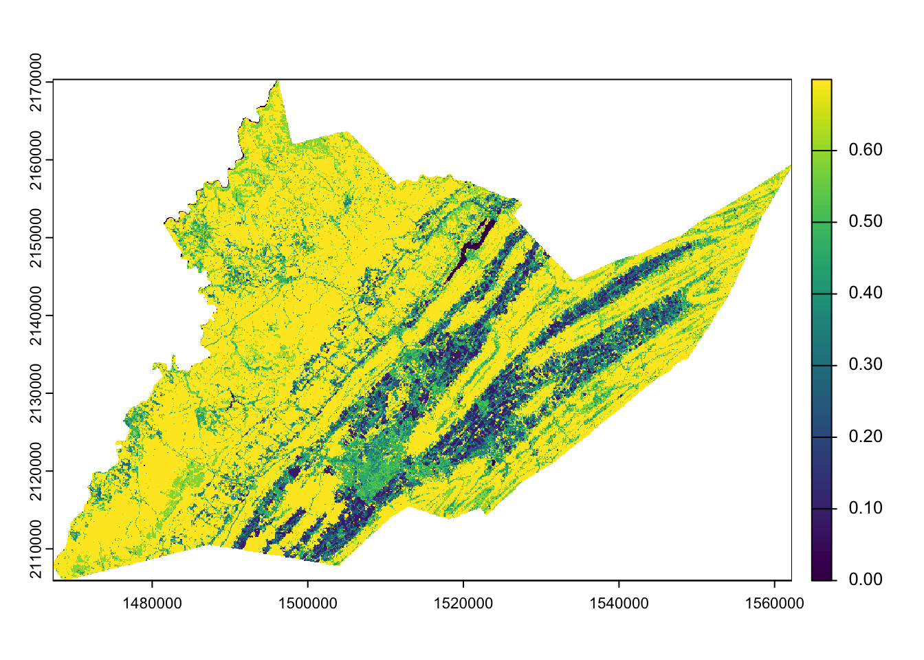
Inspect raster values
Using the values() function we can directly inspect the spring floral values for Centre County. We will set the argument na.rm=TRUE so that all the empty cells (outside of the county) are not included. The result of values() shows individual grid cell values. In this case we will only extract the first 20 grid cell values.
values(centre_floral_sp, na.rm=TRUE)[1:20] # just the first 20 cells [1] 0.5848480 0.0000000 0.6965277 0.5848480 0.0000000 0.0000000 0.6965277
[8] 0.5848480 0.0000000 0.0000000 0.6965277 0.6965277 0.6965277 0.0000000
[15] 0.0000000 0.0000000 0.6965277 0.6965277 0.5848480 0.0000000We can also use some basic summary functions to view the distribution of floral resource values for the county.
summary(values(centre_floral_sp, na.rm=TRUE)) # make a summary with the quartiles and the mean Class_Names
Min. :0.0000
1st Qu.:0.4558
Median :0.6965
Mean :0.5813
3rd Qu.:0.6965
Max. :0.6993 hist(values(centre_floral_sp, na.rm=TRUE)) # make a basic histogram of values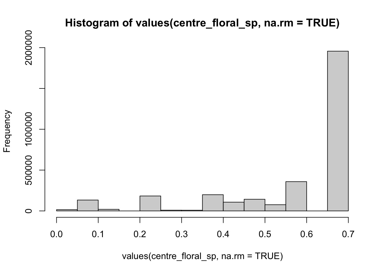
Write out raster files
We can save our raster files as a .tif using writeRaster.
writeRaster(centre_floral_sp, "data/centre_county_springfloral_2021.tif", overwrite=TRUE)